

Vector search finds the most similar items to a query by comparing high-dimensional numerical representations, called embeddings, with distance metrics. Production systems usually use approximate nearest neighbor algorithms to make that retrieval fast enough at scale.
You're probably dealing with vector search already, even if your team still calls it “AI search” or “RAG retrieval.” A support assistant needs to find the right policy despite different wording. A recommendation engine needs similar products, not products sharing the same title. A financial application needs to retrieve documents by meaning while preserving exact identifiers and access rules.
Vector search emerged from approximate nearest neighbor research that became broadly practical in the 2010s. NMSlib was the first package to include HNSW in 2016, HNSW was introduced by Malkov and Yashunin in 2016, and HNSWlib later became the reference implementation in 2018, as documented in this 2024 review of approximate nearest neighbor search. The same review notes that ANN-benchmarks compares about 50 implementations, while the Big-ANN challenge expanded evaluation to 6 datasets containing 1 billion vectors each.
The commercial direction is just as clear. An OpenSearch 451 Research report on vector evaluation says 42% of respondent enterprises already had vector-supported databases in use or in an active proof of concept. Its market context cites a 41.9% compound annual growth rate for the vector database market through 2030. Another market estimate projects the vector search market from $3.1 billion in 2025 to $32.8 billion by 2034, at a 28.5% compound annual growth rate. Those figures don't prove that every team needs a vector database, but they do show that vector retrieval has moved into mainstream infrastructure decisions.
Why Keyword Search Falls Short and Vector Search Steps In
A developer building customer support search often sees the same failure first. Someone searches “laptop won't turn on,” but the best troubleshooting article uses “black screen,” “no power,” or “device fails to boot.” A keyword engine may return weak matches or no useful result because the words differ, even though the underlying problem is the same.
Traditional lexical retrieval, including BM25 and TF-IDF, scores documents largely through terms and their weights. That behavior is valuable when the query contains an exact part number, error code, order identifier, or regulatory code. It becomes less reliable when users paraphrase, misspell, use internal jargon, or describe a concept indirectly.
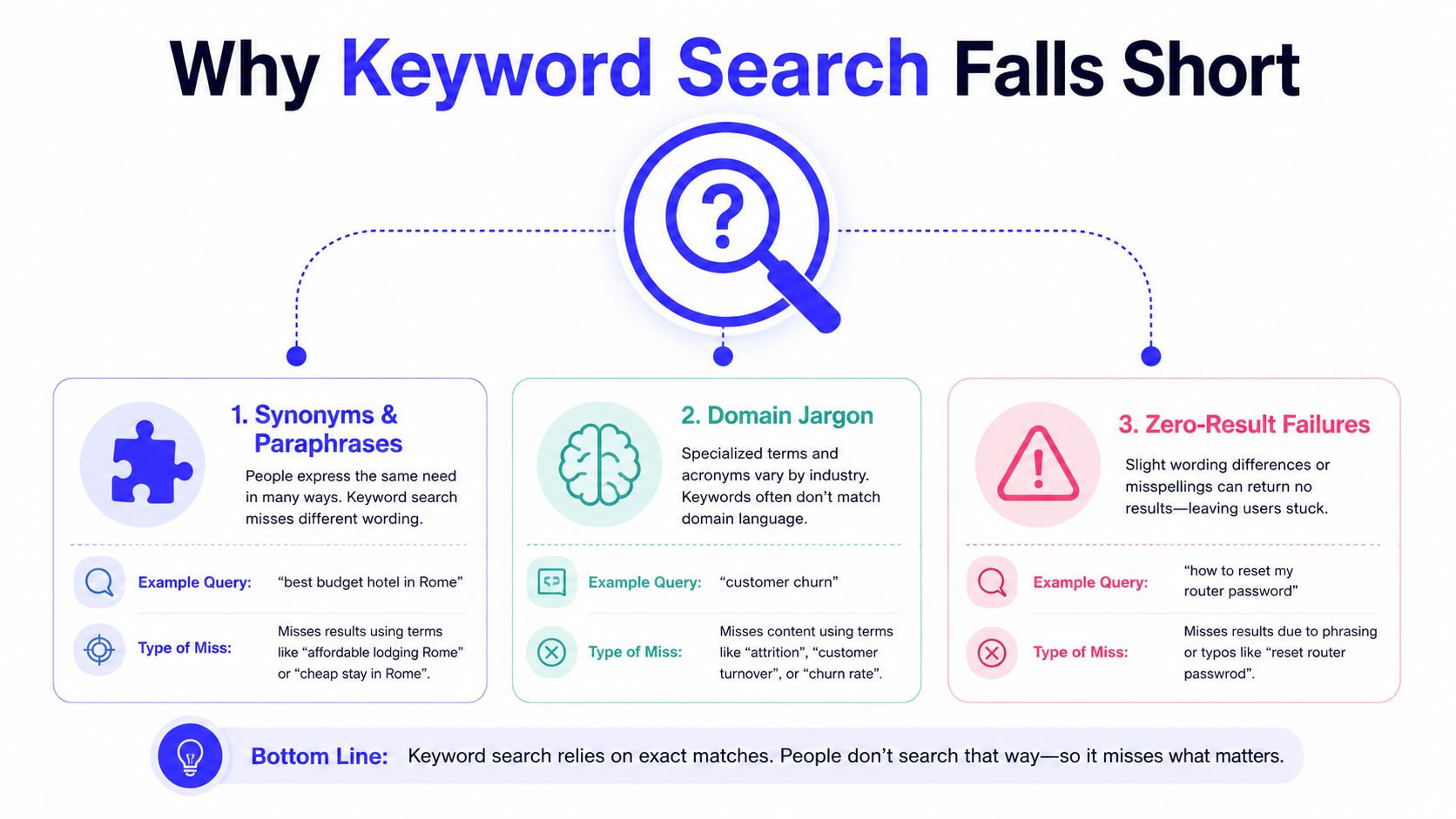
The mental model
An embedding model converts text, images, audio, or other content into a numerical representation. Items with related meaning tend to occupy nearby positions in that vector space. A query such as “my notebook has no power” can therefore retrieve content about a “black screen” even when those exact terms don't overlap.
Vector search compares the query embedding with stored embeddings using a distance or similarity metric. It then returns the nearest candidates. At small scale, the system can compare the query with every stored vector. At larger scale, an approximate nearest neighbor index narrows the search to promising regions, trading some recall for practical latency.
The distinction from keyword search is easiest to see across three dimensions:
- Synonyms and paraphrases: Dense embeddings can connect “refund pending” with an article titled “payment reversal delays.”
- Cross-lingual retrieval: Multilingual embedding models can place related content from different languages near one another, depending on model quality and domain coverage.
- Noisy queries: Semantic retrieval can tolerate informal descriptions better than strict term matching, although it won't fix poor chunking or a weak embedding model.
Why hybrid search usually wins
Vector search shouldn't replace lexical retrieval. Exact terms remain essential for product codes, legal references, software versions, names, and identifiers that embedding models may blur together. A hybrid system combines sparse keyword results with dense vector results, then merges or reranks them.
For a support assistant, a useful pattern is:
- Run keyword retrieval for exact error codes and product names.
- Run vector retrieval for paraphrases and conceptual matches.
- Apply permission and metadata filters.
- Rerank the combined candidates.
- Pass only the strongest evidence to the language model.
That pattern also helps you choose between retrieval and model customization. If the issue is stale or poorly retrieved knowledge, improve the retrieval layer before considering LLM fine-tuning versus RAG.
How Vector Search Works Under the Hood
A production vector search system has three connected layers: embeddings, indexing, and retrieval. Each layer creates constraints for the next. A strong index can't compensate for embeddings that fail to represent your domain, and a good model can't rescue an index tuned only for speed.
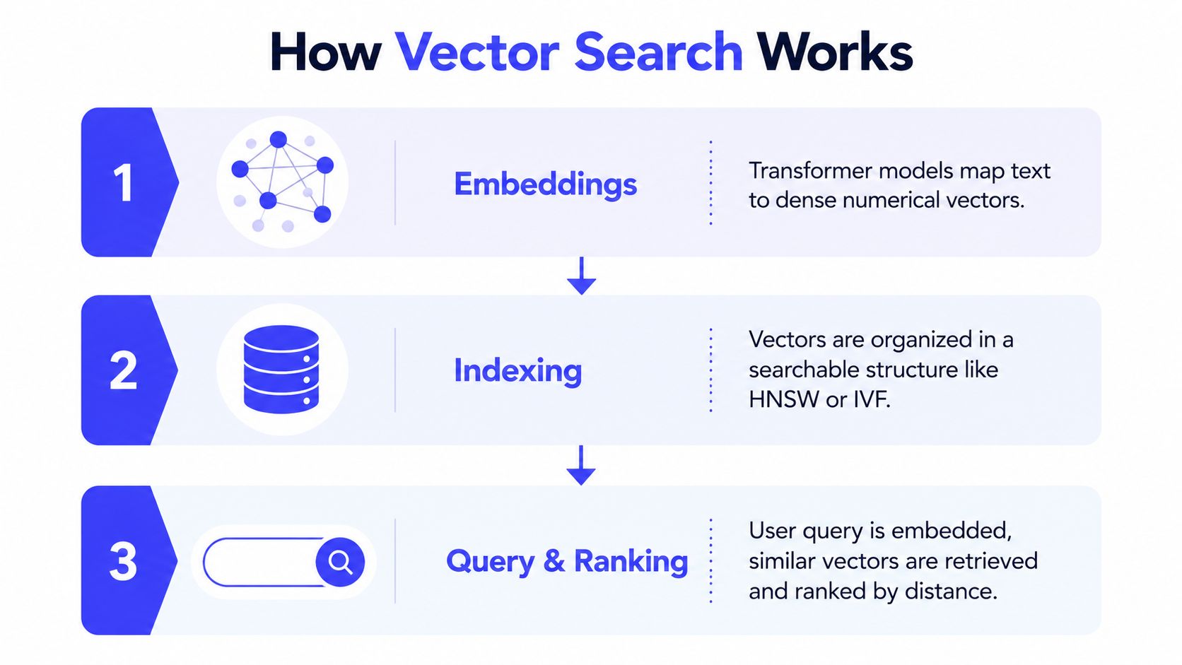
Layer one, embeddings
An embedding model maps an input into a fixed-length array of floating-point values. Transformer-based models such as OpenAI text-embedding-3, BGE, and Cohere embedding models can represent text. Other models represent images or audio.
The model choice affects more than semantic quality. Embedding dimension affects storage, memory bandwidth, and distance computation. A 384-dimensional representation behaves differently from a 1536-dimensional or 3072-dimensional representation. Higher dimensionality can preserve more information, but it also increases the cost of storing and comparing vectors. Treat dimension as an architectural decision, not a setting you can ignore until launch.
Your ingestion pipeline should version the model, preprocessing rules, chunking policy, and document identity. If any of those change, you need a controlled way to compare old and new retrieval behavior.
Layer two, indexing
The index turns a collection of vectors into a structure that can be searched efficiently. Two common families are Hierarchical Navigable Small World, or HNSW, and Inverted File with Product Quantization, or IVF-PQ.
HNSW is a graph with multiple navigable layers. A useful analogy is a library with express walkways on upper levels and detailed paths between nearby shelves below. Search starts with broad jumps and then moves through local neighbors. HNSW often offers a strong speed and recall trade-off, but it can require substantial memory and careful build tuning.
IVF first groups vectors into clusters. At query time, it identifies nearby clusters and searches only selected regions. Product quantization compresses stored vectors, which can reduce memory pressure while introducing additional approximation.
Layer three, retrieval and ranking
A query passes through a predictable path:
- The application receives the user query.
- The embedding service generates a query vector.
- The index traverses candidate regions or graph links.
- The system returns top-k candidates.
- Metadata filters, hybrid merging, and reranking refine the result.
- A downstream application uses the selected documents or items.
Operational outcomes emerge at every point. Embedding generation contributes latency and service dependency. Index configuration controls candidate quality and search cost. Filtering can change which candidates remain eligible. Reranking improves ordering but adds compute.
For teams working with specialized content, a practical introduction to natural language processing in finance can help clarify why general semantic representations may need domain-specific evaluation.
Choosing Between Exact and Approximate Search
Exact k-nearest neighbor search compares a query against every stored vector and returns the true nearest neighbors. It guarantees perfect recall, but its cost grows linearly with corpus size. That makes it valuable as a baseline and recall oracle, especially while you build a representative evaluation set.
Approximate nearest neighbor search avoids exhaustive comparison. It returns very close candidates, but the result may not contain the mathematically nearest item. Production systems commonly tune ANN retrieval toward about 95% to 99% recall, according to this comparison of approximate and exact vector search. The right target depends on whether a missed candidate harms a support answer, a recommendation, or a safety-sensitive workflow.
Distance metrics
Cosine similarity measures the angle between vectors and ranges from -1 for opposite directions to 1 for identical directions, as described in this vector search metric guide. It's common for text embeddings because it focuses on orientation rather than magnitude.
Euclidean distance measures straight-line separation. Inner product measures alignment while also incorporating vector magnitude. Dot product becomes equivalent to cosine similarity when embeddings are normalized to unit length. If your model already emits normalized vectors, dot product can be an efficient choice. If vector length carries unwanted bias, cosine similarity is safer.
Vector Search Strategy Decision Matrix
| Workload Factor | Brute-Force k-NN | HNSW | IVF-PQ | ScaNN |
|---|---|---|---|---|
| Dataset size | Strong fit for small corpora, often under 100k vectors | General-purpose choice as the corpus grows | Useful when the corpus and memory footprint are large | Useful when the team can support specialized tuning |
| Latency budget | Simple but becomes expensive as data grows | Good candidate for general-purpose queries under 50ms, subject to hardware and workload | Can provide efficient search with compression and cluster probing | Designed for high-throughput approximate retrieval |
| Recall requirement | Best baseline and perfect-recall reference | Tune ef_search upward for more candidates and recall | Tune nprobe upward to inspect more clusters | Tune partition and candidate settings against a ground-truth set |
| Filter selectivity | Predictable when filters sharply narrow the set | Can degrade when filters exclude most graph candidates | Can degrade when relevant filtered items span clusters | Requires workload-specific benchmarking |
| Memory pressure | Stores full vectors and scans them | Usually higher memory use than compressed approaches | Product quantization reduces memory at the cost of approximation | Depends on implementation and compression choices |
The thresholds in the table are decision heuristics, not guarantees. Hardware, dimension, filters, and query concurrency can move the crossover point.
Practical rule: Build an exact-search baseline first. Then increase ANN speed gradually while measuring recall against that baseline.
Default settings usually favor convenience or throughput. For HNSW, ef_search controls how much of the graph the query explores. For IVF, nprobe controls how many clusters it examines. Raising either generally improves candidate coverage while increasing query work. Tune these settings against production-like queries, not a handful of clean examples.
Production Architectures and Tool Stacks
A small internal knowledge base and a high-volume recommendation engine may both use vector search, but they shouldn't share the same architecture by default.
For an internal RAG application, a practical first version might use an OpenAI embedding model, Pinecone or Weaviate, and LangChain for orchestration. The ingestion path extracts documents, applies a chunking policy, generates embeddings, and writes vectors with metadata such as source, access group, document version, and update time. The query path embeds the user's question, retrieves candidates, applies permissions, reranks, and sends grounded context to the language model.
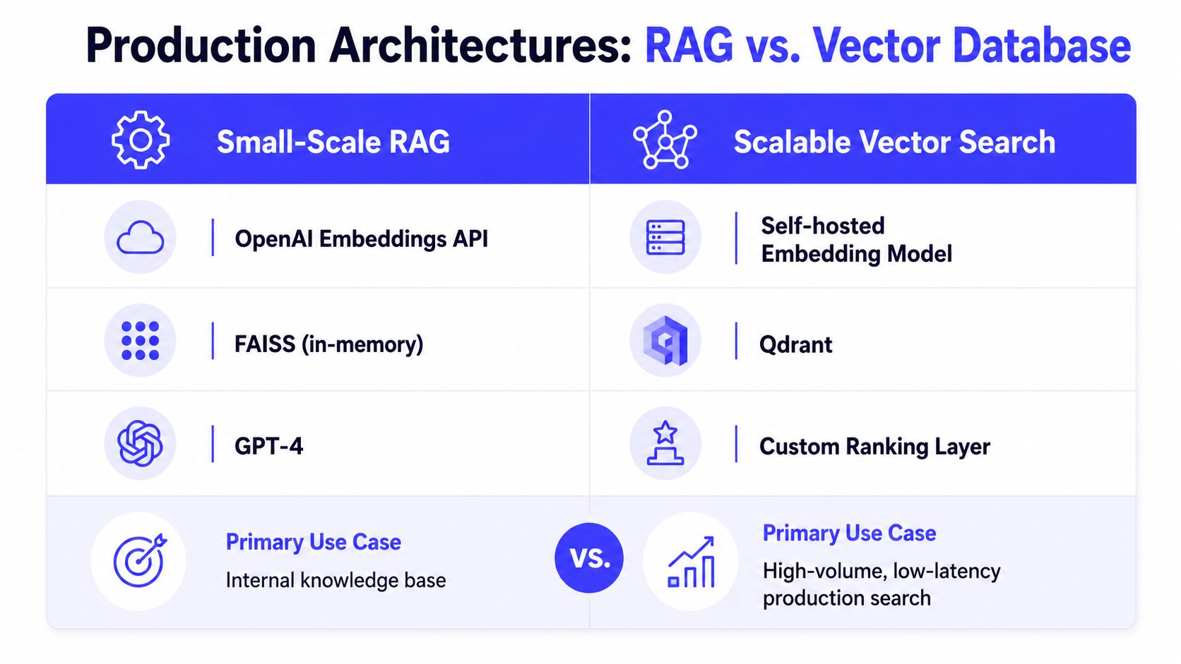
Example one, internal RAG
The first bottleneck often isn't the vector database. It may be embedding-service latency, oversized chunks, duplicate content, permission filtering, or a slow reranker. Large chunks can contain the right answer but bury it among unrelated material. Tiny chunks can lose the context needed to answer accurately.
A representative design review should ask:
- Which chunking rule preserves the answer and its surrounding conditions?
- Are filters applied before retrieval, during retrieval, or after candidate generation?
- Does the system log retrieved chunk IDs and document versions?
- Can the team reproduce a poor answer from the original source state?
A managed database reduces cluster operations and makes a pilot easier. The trade-off is less control over index internals, pricing, and migration paths. The application still needs careful evaluation and governance. Vector infrastructure doesn't remove the need for sound LLM application development practices.
Example two, recommendation retrieval
A recommendation service serving a large catalog may use Milvus or Qdrant on self-hosted Kubernetes, a self-hosted BGE or E5 embedding model, product quantization for memory control, and Redis for frequently requested results. A custom ranking layer can combine vector similarity with inventory, business rules, user history, and freshness.
The difficult decisions are operational:
- Shard count: Choose enough shards for parallelism and failure isolation, but avoid creating tiny partitions that complicate balancing.
- HNSW settings: Set graph construction and search parameters from recall and latency tests, not copied defaults.
- Caching: Cache stable, high-frequency queries, but invalidate results when catalog or eligibility data changes.
- Model ownership: Self-hosted embeddings reduce provider dependency but add model serving, capacity planning, and upgrade work.
Managed services usually reduce time to a working system. Self-hosting can provide stronger control over residency, topology, and long-run unit economics, but only when the team can operate distributed storage, monitoring, upgrades, and recovery. The crossover isn't determined by vector count alone. Query volume, compliance, data churn, and engineering capacity matter just as much.
Hidden Costs and Operational Limits at Scale
A vector index is a maintained data product, not a static table. The hardest failures often arrive after the demo, when source data changes, access rules evolve, and query patterns become unpredictable.
Embedding drift is one major risk. If you change the embedding model or its preprocessing, old vectors and new query vectors may no longer occupy a compatible space. You may need to re-embed the corpus, validate retrieval quality, and migrate indexes without exposing inconsistent results. A 2025 industry review highlights embedding drift, real-time ingestion, memory trade-offs, and index maintenance as active production problems, and notes that mainstream platforms have reduced vector index build time by up to 20x, which itself shows how important indexing efficiency remains (industry review of vector search developments).
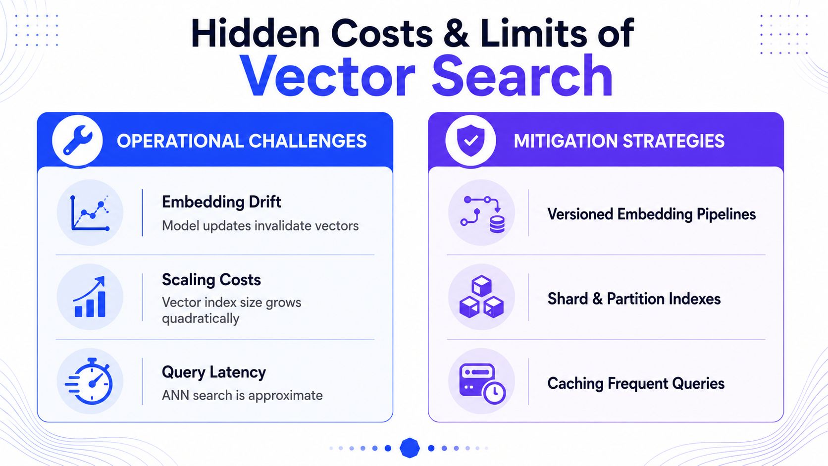
Freshness and write pressure
HNSW is built primarily for efficient navigation during search. Heavy streaming inserts, updates, and deletes can increase maintenance work and destabilize latency. An ingestion design commonly separates incoming data from the serving index, batches updates where possible, and supports blue-green or versioned index replacement.
You also need an explicit source-of-truth policy. When a document changes, the system should know whether to update one chunk, reprocess the full document, remove stale chunks, or retain historical versions for audit.
Filters can erase ANN gains
Filtered vector search is more complicated than “find similar items where category equals X.” A highly selective permission or date filter may exclude the candidates that an ANN index finds quickly. The engine may need to explore more candidates or fall back toward broader scanning.
The filtered vector search tutorial from VLDB 2025 identifies unresolved issues around autotuning, index choice, quality metrics, and benchmarking. That means you should benchmark filters as part of retrieval quality, not add them after an unfiltered ANN test.
Memory planning also needs discipline. One billion 1536-dimensional float32 vectors require roughly 6TB of RAM before indexing structures, based on the raw vector representation. Compression, sharding, tiered storage, and dimensionality choices can change the design, but none removes the need for a capacity model.
A successful pilot proves relevance on a sample. Production proves freshness, permissions, recovery, and cost under change.
Monitor retrieval quality alongside infrastructure metrics. Track query latency percentiles, empty-result rates, filter rejection rates, index age, embedding version, and human or downstream feedback. Teams often detect silent quality degradation only after users stop trusting the search experience. For broader latency and serving considerations, see this guide to AI inference optimization.
Evaluation Metrics and Deployment Patterns
A vector search system works only if it retrieves useful candidates under the conditions your application creates. Vendor benchmarks can help compare implementations, but they won't represent your documents, filters, languages, update patterns, or query distribution.
Start with a labeled query set. For each query, record acceptable documents or items, required permissions, and the downstream outcome. Then compare exact search with your ANN configuration and test both filtered and unfiltered paths.
Metrics that connect retrieval to value
Recall@k measures how many of the true nearest neighbors appear in the returned top-k set. It tells you whether the index is finding the right neighborhood, but it doesn't guarantee that the first result is useful to a person.
Latency should be measured at p50, p95, and p99 under realistic concurrency. RAG systems should add answer accuracy or groundedness checks. Recommendation systems should add business-facing behavior metrics such as click-through rate, while recognizing that user behavior can be influenced by ranking, presentation, and inventory.
Vector Search Evaluation Metrics and Targets
| Metric | Definition | RAG Target | Recommendation Target | Measurement Frequency |
|---|---|---|---|---|
| Recall@k | Fraction of true nearest neighbors present in top-k | Set from exact-search baseline and answer-quality needs | Set from offline relevance labels and downstream tests | Every index or model change |
| p50 latency | Median request latency | Must support the product's interactive experience | Must meet serving budget for the recommendation surface | Continuous |
| p95 latency | Latency below which most requests fall | Test with filters, reranking, and embedding generation included | Test during realistic traffic and catalog conditions | Continuous |
| p99 latency | Tail latency for the slowest requests | Use to detect permission and cold-partition problems | Use to detect shard imbalance and cache misses | Continuous |
| Downstream quality | Accuracy of the final application outcome | Human or automated grounded-answer evaluation | Offline relevance plus online behavior evaluation | Per release and scheduled review |
Deployment maturity should follow evaluation maturity:
- Managed first: Use a managed service when speed to a reliable prototype matters more than infrastructure control.
- Hybrid next: Keep managed embeddings while self-hosting or optimizing the index when cost, residency, or integration needs increase.
- Self-hosted selectively: Operate Milvus, Qdrant, or another stack only when the workload justifies the operational surface area.
Managed services still need a strong machine learning engineer for embedding selection, query design, evaluation, and reranking. Self-hosting adds requirements for Kubernetes, capacity planning, distributed systems, observability, backup, and incident response. Buying the database doesn't eliminate expertise. It changes where that expertise is applied.
Building Your Team and Getting Started
The build-versus-buy decision is partly a staffing decision. Integration work needs engineers who can select embeddings, design chunks, orchestrate RAG, write evaluation sets, and connect retrieval to application behavior. A deep infrastructure build needs additional skill in ANN algorithm tuning, distributed indexing, storage layout, custom distance functions, and operational recovery.
A practical hiring checklist
- Retrieval engineer: Can compare embeddings, create labeled queries, diagnose misses, and tune reranking.
- ML engineer: Can serve or integrate embedding models and connect retrieval quality to downstream outcomes.
- Platform or MLOps engineer: Can automate ingestion, model versioning, monitoring, reindexing, and rollback.
- Application engineer: Can enforce permissions, expose citations, handle failures, and instrument user feedback.
- Technical lead: Can decide whether managed infrastructure or self-hosting fits the team's risk and capacity.
An eight-week pilot
Weeks 1–2: Prepare representative data, define document and permission rules, evaluate embedding models, and create a labeled query set.
Weeks 3–4: Prototype with a managed service such as Pinecone or Weaviate. Compare chunking, metadata schemas, hybrid retrieval, and reranking.
Weeks 5–6: Benchmark recall and latency using realistic filtered queries. Compare exact retrieval with HNSW or IVF-PQ configurations, then test ingestion and update behavior.
Weeks 7–8: Harden the service. Add index versioning, embedding-drift monitoring, reindexing workflows, access-control tests, dashboards, and rollback procedures.
A team can consider moving toward Milvus or Qdrant when infrastructure control, residency, or workload economics justify the burden. A useful planning signal is around 50M+ vectors, but it isn't a universal threshold. Query volume, update frequency, compliance requirements, memory costs, and available operators should determine the decision.
Run these three actions this week:
- Collect representative queries and label acceptable results.
- Build an exact-search baseline before tuning ANN settings.
- Interview candidates with a retrieval debugging exercise, not only a generic machine learning quiz.
ThirstySprout helps teams hire senior AI engineers and remote ML teams for vector search, RAG, embedding pipelines, and MLOps work. If you need practical help evaluating a managed stack or building the people and systems around it, visit ThirstySprout to start a pilot or see how the network can support your next production search project.
Hire from the Top 1% Talent Network
Ready to accelerate your hiring or scale your company with our top-tier technical talent? Let's chat.