

Monday morning. The growth team wants a cleaner A/B testing workflow, finance needs a forecast they can audit, and engineering is pushing to standardize on Python because it feels safer operationally. The core decision is narrower than that debate suggests. Which parts of your data workflow need fast statistical iteration, readable analysis code, and reporting your stakeholders can readily review?
R is a good fit for that slice of work. It is less compelling as a general application language, but it remains strong for statistical modeling, time-series forecasting, experiment analysis, reproducible reporting, and analyst-facing apps. For a CTO or tech lead, that trade-off matters because it affects hiring, deployment complexity, and time-to-value.
This article focuses on 8 production-grade R programming language examples, not toy scripts. The goal is to show where R earns its place in a modern stack, where Python is still the better operational choice, and how teams at larger companies use R patterns for work that directly impacts forecasting accuracy, experimentation speed, reporting reliability, and model governance.
R was created for statistical computing and graphics, and that origin still shows up in the workflows it handles well. You see it in feature engineering pipelines, in experimentation frameworks, and in reporting systems where reproducibility matters as much as raw model performance. If your team is evaluating feature engineering methods for machine learning workflows, R is often strongest where transformation logic, statistical assumptions, and business review need to stay close together.
The sections that follow are written from a production lens. Each example includes code, the operational trade-offs, and the business case for using R instead of defaulting to Python everywhere.
1. Data Cleaning and Transformation Pipeline with dplyr for ML Feature Engineering
Messy data is where most ML timelines slip. R is especially good when your team needs readable transformation logic that analysts, data scientists, and reviewers can all inspect without digging through a large application codebase.
A practical pattern is to use dplyr and tidyr to build one chained pipeline that cleans fields, standardizes types, and creates features in a reproducible order. In e-commerce, that usually means deriving purchase frequency, recency, and device-level behavior from raw transaction logs. In fintech, it often means filling missing transaction amounts carefully, flagging extreme values for review, and creating lagged variables for forecasting or fraud screens.
A production pattern
library(dplyr)library(tidyr)library(lubridate)features <- raw_txn %>%mutate(event_time = ymd_hms(event_time, tz = "UTC"),amount = if_else(is.na(amount), 0, amount),device_type = replace_na(device_type, "unknown")) %>%distinct(user_id, event_time, .keep_all = TRUE) %>%group_by(user_id) %>%arrange(event_time, .by_group = TRUE) %>%mutate(txn_lag_1 = lag(amount),purchase_count = n(),total_spend = sum(amount, na.rm = TRUE),avg_spend = mean(amount, na.rm = TRUE)) %>%ungroup()This works well for SaaS product analytics too. If data arrives from many APIs, standardize timestamps first, deduplicate aggressively, and aggregate to the business grain you'll model against, such as daily account activity or weekly cohort retention.
What works and what breaks
A few habits make these pipelines production-safe.
- Use helper selectors early:
select(starts_with("feat_"))orselect(ends_with("_ts"))keeps wide datasets manageable when you're carrying many engineered columns. - Apply transforms consistently:
mutate(across(where(is.numeric), log1p))is cleaner than repeating the same line across many fields. - Validate at every boundary:
glimpse(),count(), and a small sampled export catch silent type issues before they leak into training jobs. - Push large joins to the warehouse: database-backed tibbles keep memory usage under control and shorten failure recovery.
Practical rule: If your feature logic isn't readable in one pass, your future debugging cost will be higher than your current coding speed.
Feature engineering itself is often where business value appears or disappears. If you're mapping raw events into model-ready inputs, this feature engineering in machine learning guide is worth keeping nearby for team reviews.
2. Statistical Hypothesis Testing and A/B Testing Framework with tidymodels
A PM asks for a green light on a pricing test after five days because the dashboard shows a lift. That is usually where teams create avoidable risk. If the assignment is uneven, the window is too short, or repeated user behavior is ignored, the rollout decision can cost more than the experiment saved.
R remains a strong choice for this class of work because the language was built around statistical modeling, not added to it later. For CTOs comparing R with Python, that matters most when the question is causal inference, test design, and reviewability under pressure. Python often wins on broader platform standardization. R often wins on speed to a correct experimental analysis for analysts and statisticians already working in that stack.
A reusable experiment skeleton
library(dplyr)library(infer)set.seed(42)results <- experiment_df %>%specify(conversion ~ variant) %>%hypothesize(null = "independence") %>%generate(reps = 1000, type = "permute") %>%calculate(stat = "diff in props", order = c("treatment", "control"))The code is simple on purpose. The production value comes from the surrounding process. Store the hypothesis, owner, exposure rule, primary metric, analysis window, and stopping criteria with the result so another analyst can reproduce the call without reverse-engineering a notebook two months later.
For SaaS onboarding tests, this pattern works well when the metric is binary and assignment is clean. In fintech collections or reminder-message tests, add controls for repeated observations and cohort effects before anyone interprets a lift as causal. Teams that skip that step usually end up debating instrumentation instead of deciding what to ship.
A review standard that holds up in production looks like this:
- Estimate sample size before launch: use power analysis up front so the team knows whether the experiment can answer the business question in the available time.
- Start with intent-to-treat: analyze users by assigned variant first. Per-protocol cuts can help diagnose behavior, but they should not drive the main decision.
- Report effect size with uncertainty: confidence intervals and expected business impact are more useful to executives than a single p-value.
- Log baseline covariates: country, device class, plan tier, or prior activity often explain more variance than teams expect.
- Define guardrails early: revenue per user, support contacts, repayment behavior, or churn can block rollout even when the primary metric improves.
One more trade-off is worth calling out. infer and the tidymodels style make experiment code readable and teachable, which lowers review time for mixed teams. If you need highly customized Bayesian workflows or very large-scale online experimentation infrastructure, you may outgrow this pattern and move parts of the stack elsewhere. That does not reduce R's value for pilot programs, retrospective analysis, or high-stakes tests where statistical correctness matters more than framework uniformity.
For teams pairing experimentation with operational monitoring, this guide to detecting anomalies in time series is a useful complement. It helps separate treatment effects from traffic spikes, outages, and seasonality that can distort short test windows.
What fails in practice is not the hypothesis test itself. It is weak experiment hygiene. Pricing, risk, and rollout decisions need an analysis path that another engineer, analyst, or auditor can rerun without guessing what happened.
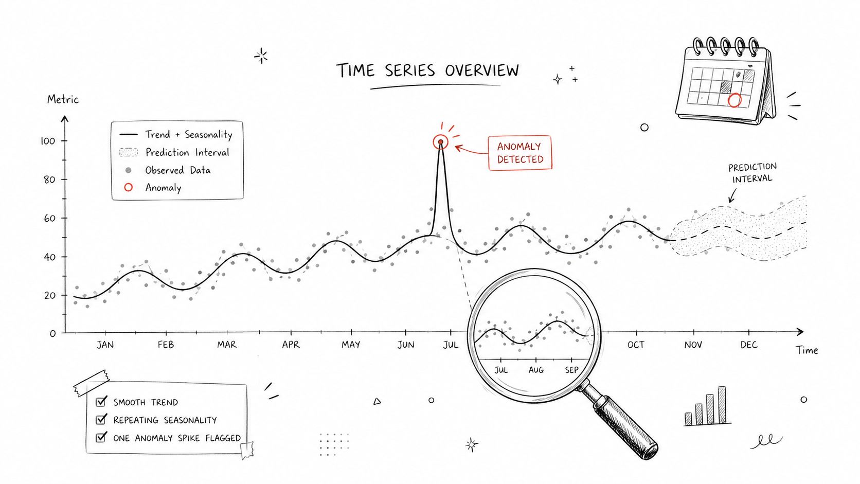
3. Time-Series Forecasting and Anomaly Detection with Prophet and fable
Forecasting is one of the clearest places where R earns its keep. Finance teams, operations leads, and growth teams often need reliable answers fast, not a sprawling platform rebuild.
For SaaS, that might mean projecting monthly recurring revenue and flagging unexpected churn spikes. In e-commerce, it could be per-SKU demand planning before a seasonal event. In fintech, it's often transaction volume forecasting so infrastructure and fraud operations can staff appropriately.
Here's the visual shape of the problem commonly solved:
A forecasting pattern that holds up
library(fable)library(tsibble)library(dplyr)fc <- revenue_ts %>%model(arima = ARIMA(revenue)) %>%forecast()That's deliberately simple. In production, the harder part is handling changepoints, outages, promotions, and holidays without contaminating the baseline. Prophet and fable both help, but neither saves you from weak operational assumptions.
R is widely used in finance for time-series work. ANZ Bank used R for credit risk analysis and portfolio management, relying on time-series methods such as moving averages and autoregression, as described in DataFlair's roundup of R applications. That's the right mental model for CTOs. Use R where time-aware statistical reasoning is central to the business decision.
Operational guidance
- Hold out recent history: keep the latest period untouched for a realistic backtest.
- Record major business events: launches, outages, and pricing changes should be logged alongside the data.
- Alert with rules, not model output alone: consecutive out-of-band periods are usually more actionable than a single noisy spike.
- Turn anomalies into workflows: route them to ops owners, not just a chart.
If anomaly detection is part of your stack review, this time-series anomaly detection guide helps connect the modeling decision to operational alerting.
A forecast is only useful if someone knows what to do when it's wrong.
4. Machine Learning Model Development and Evaluation with caret and mlbench
A familiar production scenario. The growth team wants a churn model in two weeks, compliance wants a model card, and engineering wants something they can rerun without a month of framework decisions. caret is a practical choice for that kind of work. It gives R teams one consistent training interface across multiple algorithms, which lowers setup time and makes side-by-side comparison easier.
That matters when the actual decision is not "can we train a model?" but "which workflow gets us to a defensible baseline fastest?" For tabular supervised learning, R still holds up well. caret is older than newer toolchains, but that can be an advantage in stable enterprise environments where predictability matters more than novelty.
A straightforward model training setup
library(caret)set.seed(42)idx <- createDataPartition(df$target, p = 0.8, list = FALSE)train_df <- df[idx, ]test_df <- df[-idx, ]ctrl <- trainControl(method = "cv",savePredictions = "final",classProbs = TRUE)model <- train(target ~ .,data = train_df,method = "rf",trControl = ctrl)This pattern fits common business cases such as churn prediction, credit risk scoring, lead qualification, and fraud triage. It is also useful when a team needs to compare logistic regression, random forest, and gradient boosting on the same feature set without rewriting the surrounding workflow. That consistency cuts analyst time and reduces review friction.
mlbench is useful here because it gives teams standard datasets for testing training code, resampling logic, and evaluation templates before they point the workflow at sensitive production data. I often recommend that step for teams piloting R. It surfaces issues in factor handling, missing values, and metric selection early, when the cost of mistakes is still low.
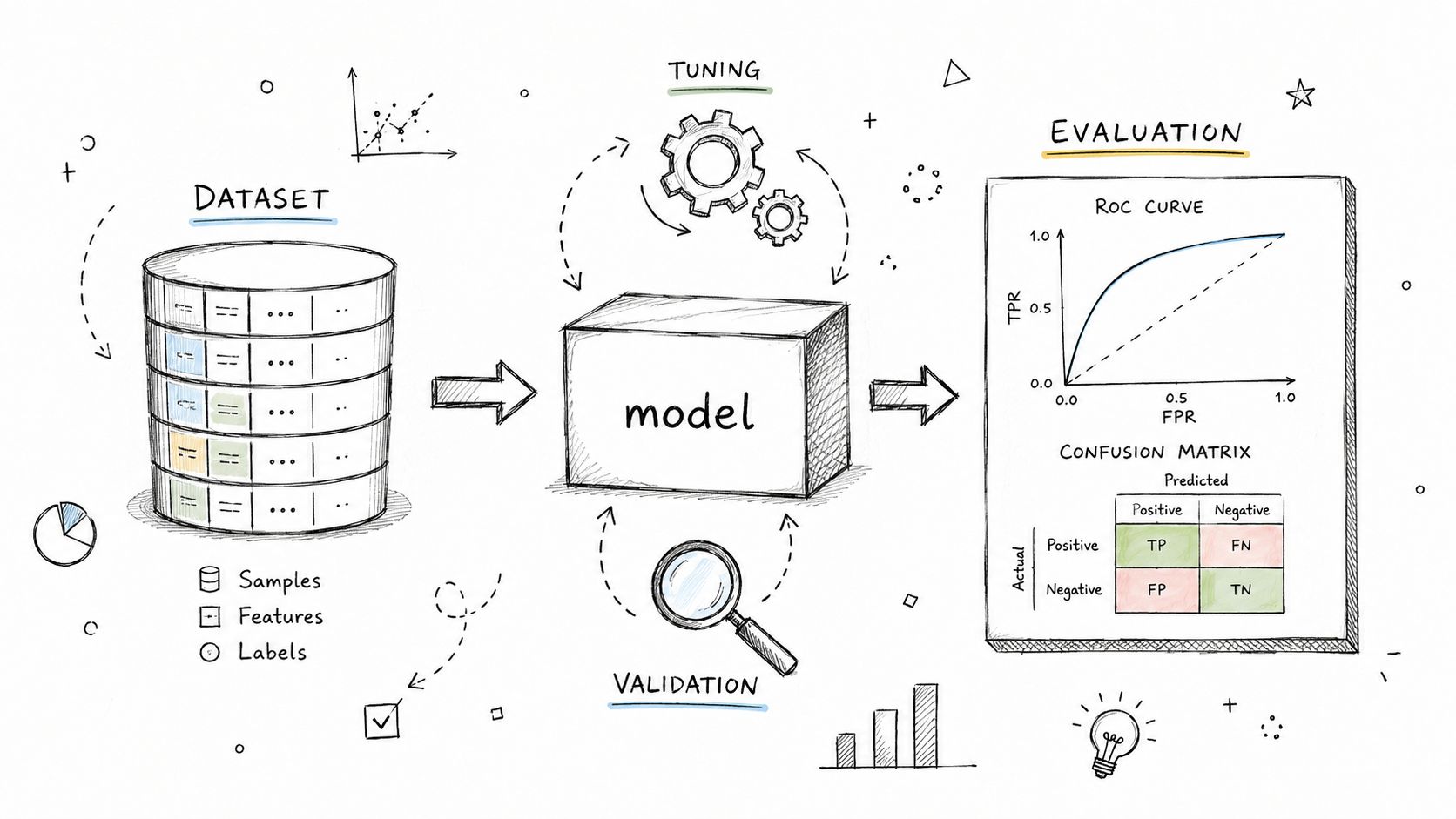
What good evaluation looks like
R's package ecosystem gives teams broad modeling coverage, which is useful when a business problem needs specialized methods. The trade-off is governance. More package choice means more work on version control, security review, and long-term maintenance. For a CTO, that is the core evaluation question. Model quality matters, but supportability matters too.
Keep the evaluation standard tight:
- Preserve class balance: use stratified splits for rare outcomes so recall estimates are not distorted.
- Match thresholds to business cost: if missing fraud is ten times more expensive than reviewing a false alert, optimize for that reality.
- Protect the holdout set: use it once for the final estimate, not as a tuning crutch.
- Review feature stability: importance rankings can shift when correlated predictors or policy-driven fields enter the training data.
- Test for operational fit: score latency, batch throughput, and reproducibility should be checked before rollout, not after sign-off.
A model with a slightly lower AUC but clearer behavior, easier retraining, and fewer deployment dependencies often wins in production. That is especially true in regulated domains, where auditability and failure handling affect delivery time as much as raw predictive performance.
5. Interactive Data Visualization and Dashboards with Shiny and plotly
A common pattern in data teams is easy to spot. The model exists, the SQL exists, the business question is clear, but decisions still wait because nobody has turned the analysis into a tool that operations, finance, or product can use daily. Shiny closes that gap faster than a custom frontend for many internal workflows.
That speed matters when the dashboard is tied to revenue or risk. I've seen Shiny work well for churn review portals, experiment readouts for product managers, and model-monitoring consoles where teams need segment-level drill-downs without adding another application project to the roadmap. The trade-off is straightforward. Shiny reduces time-to-value, but once usage grows, the app needs the same engineering discipline as any internal product.
A rough picture of the end state helps align non-engineering stakeholders:
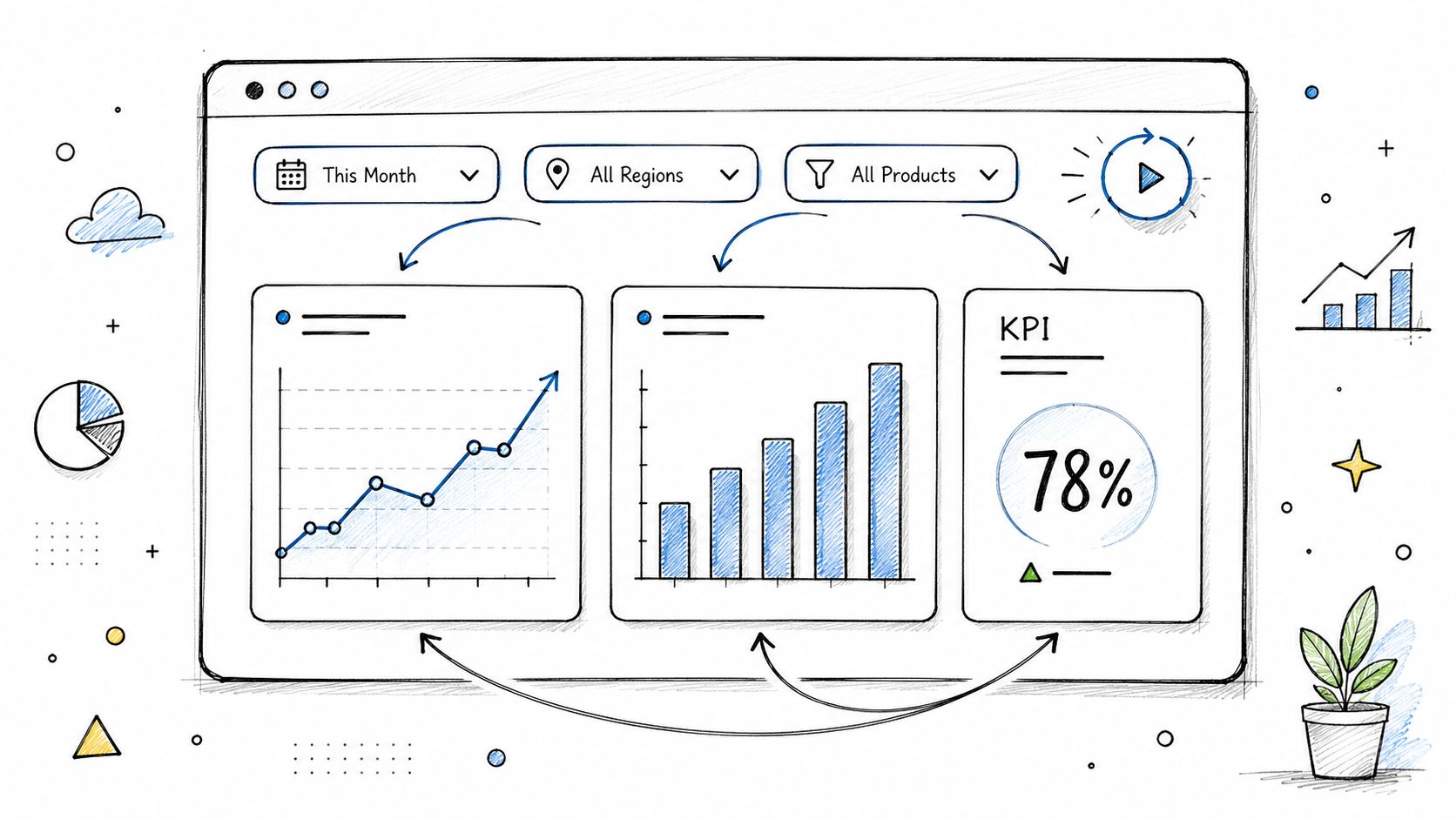
A lean Shiny pattern
library(shiny)library(plotly)ui <- fluidPage(selectInput("segment", "Segment", choices = c("all", "enterprise", "smb")),plotlyOutput("trend_plot"))server <- function(input, output, session) {filtered <- reactive({subset(metrics_df, segment == input$segment | input$segment == "all")})output$trend_plot <- renderPlotly({plot_ly(filtered(), x = ~date, y = ~value, type = "scatter", mode = "lines")})}shinyApp(ui, server)This pattern is useful because it keeps the first release small. A team can validate whether stakeholders use segment filters, drill-downs, and weekly trend views before investing in a larger BI build or a React application.
For CTOs comparing R with Python, this is one of R's stronger positions. If the core team already works in R, Shiny usually gets an internal analytical app into users' hands faster than rebuilding the same workflow in Flask or FastAPI plus a JavaScript frontend. Python gives more flexibility for broader application platforms. R often wins for analyst-led decision tools where the charting logic, statistical context, and app behavior live close together.
The architecture choices matter more than the widget library. Keep heavy filtering and aggregation in the warehouse or database. Cache expensive queries. Treat reactive expressions as application state, not as a place to hide business logic. If the app becomes part of an operating process, package it, containerize it, set request and memory limits, and log usage and failures the same way you would for any internal service.
plotly adds practical value here because users can inspect points, zoom into anomalies, and compare segments without asking an analyst for a new static export. That lowers reporting overhead. It also creates a governance question. Interactive dashboards make it easy to expose unstable metrics, so teams need clear metric definitions and refresh rules before rollout.
If the dashboard output needs to move into executive reporting, procurement reviews, or client deliverables, pair the Shiny workflow with export paths that non-technical teams can use. For document handoff, flawless Markdown to DOCX conversions can save time when charts and written analysis need to leave the app and enter a formal approval process.
A short product demo helps teams understand what “good enough for internal use” looks like:
6. Reproducible Research and Report Generation with R Markdown and Quarto
A familiar failure mode looks like this. The model output is right, the slide deck is wrong, and nobody can trace which SQL extract, feature set, or parameter choice made it into the final recommendation. R Markdown and Quarto fix that problem well because they tie code, narrative, tables, and charts into one build artifact.
That matters in production settings where reports are part of the decision path, not just analyst output. Teams use these workflows for monthly churn reviews, risk committee packs, experiment readouts, and model validation documents that need a clean audit trail. For a CTO, the value is simple: less manual reconciliation, faster review cycles, and lower risk that a copied chart or stale assumption survives into an executive decision.
A report pipeline that teams actually reuse
---title: "Monthly Model Report"format: htmlparams:model_version: "v1"report_date: "2026-07-01"---summary_tbl <- predictions |>dplyr::group_by(segment) |>dplyr::summarise(avg_score = mean(score, na.rm = TRUE))Parameterized reports are what make this operational instead of academic. One template can render by region, customer segment, reporting date, or model version, which cuts copy-paste drift and keeps review logic consistent across the business.
The production pattern I recommend is straightforward. Keep .Rmd or .qmd files in Git. Render reports in CI or a scheduled job. Store large HTML, PDF, or DOCX outputs in artifact storage rather than the repo. Capture sessionInfo() or an equivalent environment snapshot when the document supports a pricing change, model rollout, or board-level metric.
This is also where Quarto has an edge for mixed-language teams. It handles R, Python, and SQL in one reporting workflow, which helps when an organization is comparing language choices across analytics groups. If that comparison is part of a wider delivery standard, align report generation with your MLOps workflow and deployment standards so builds, approvals, and artifact retention follow the same operating model as the rest of the stack.
Trade-offs worth knowing
R Markdown and Quarto improve trust because the path from source data to conclusion is inspectable. That benefit disappears if reports are still rendered manually on analyst laptops. The common failure is partial reproducibility: versioned templates, but unpinned packages, local file paths, and no record of which parameters were used.
There is also a cost trade-off. Highly polished document generation can pull analysts into formatting work that belongs in a standardized template. Keep the report layout stable and spend effort on parameterization, validation checks, and distribution. That gets more value than tweaking themes every quarter.
If stakeholders need editable files after technical review, tools for flawless Markdown to DOCX conversions can help bridge the handoff without rewriting the report manually.
7. Cross-cutting Production R Best Practices
Most failures with R in production aren't about the language. They come from weak packaging, poor environment control, and vague ownership boundaries.
This matters more now because teams increasingly care about deployment quality, not just modeling quality. One useful signal is the underserved gap in current R education. Mainstream tutorials still focus on beginner syntax and isolated plots, even as torch and mirai make R more relevant to modern ML and parallel workloads. The same source notes that 68% of data science teams now prioritize languages with strong production deployment capabilities, which is exactly why packaging and deployment patterns matter so much, as discussed in Efficient R's learning resources.
The operating standard I'd use
- Validate intermediate outputs:
glimpse(),count(), and small spot checks catch silent failures early. - Push heavy work down: use SQL and warehouse execution for large joins, then keep R focused on modeling and aggregation.
- Pin environments: use
renvand container builds so analysts, CI, and production don't drift apart. - Log experiment and model metadata: seeds, preprocessing steps, report parameters, and training context should all be recoverable.
- Store heavy artifacts outside Git: keep source lightweight and retrieval predictable.
Operating principle: R is excellent at analytical logic. It's less forgiving when teams treat ad hoc scripts as production services.
If you're formalizing those guardrails across your stack, this MLOps best practices guide maps well to the controls R teams usually need.
8. Enterprise Adoption and Impact Summary
A CTO usually asks this question at the point where prototypes have already worked: can R carry a production workflow without adding delivery risk? The answer is yes, in the right operating model. These examples show where R earns its place because it shortens time-to-insight, keeps statistical work close to domain experts, and turns analysis into repeatable reporting and decision support.
R is a strong fit when the highest-value work sits in forecasting, experimentation, risk analysis, regulated reporting, and dashboard-heavy internal tools. In those cases, teams often ship faster with R than with a general-purpose stack because the analytical libraries are mature and the path from notebook to report to Shiny app is short. The trade-off is clear. R is usually best as part of a broader platform, not the language that owns every service boundary.
Enterprise adoption is most credible where mistakes are expensive.
In finance, R remains common for portfolio analysis, risk measurement, and scenario modeling because packages such as PerformanceAnalytics, quantmod, and PortfolioAnalytics support workflows that need transparent math and auditable outputs. The overview of real-world R data science projects is broad, but it points to the right pattern: R tends to stay where statistical depth matters more than app-layer breadth.
Operations is another practical use case. The IJETER paper on R-based production simulation describes a discrete event simulation built with simmer to measure cycle timing in a production system. That matters because it reflects a real business workflow. Teams used R to test throughput and latency assumptions before changing processes on the floor. For a CTO, that translates into lower process risk and faster evaluation of operational changes.
R also fits well in AI-adjacent product work when the problem is still analytics-first. Teams can use R to validate experiments, generate model monitoring reports, or prototype decision logic before handing hardened services to a Python or TypeScript stack. For leaders mapping that handoff, the MeshBase blog on AI app building is a useful reference for the application side of the equation.
The decision framework is straightforward:
Choose R when statistical rigor, reporting, and analyst productivity drive the return. Choose Python when the same team must also own application services, model serving infrastructure, and a larger share of platform engineering.
That is the practical takeaway from these R programming language examples. R does not need to be the default for everything. It needs to be the fastest reliable option for the parts of the workflow where analytical correctness, iteration speed, and communication to the business matter most.
R Programming: 8-Point Comparison
| Tool / Approach | Implementation Complexity 🔄 | Resource & Scale ⚡ | Expected Outcomes ⭐ / Impact 📊 | Ideal Use Cases | Key Advantages & Tips 💡 |
|---|---|---|---|---|---|
| Data Cleaning & Transformation Pipeline (dplyr/tidyr) | Moderate, learn tidyverse grammar and pipeline patterns | Medium, efficient for 100k–1M rows; degrades >2GB without DB/parallel backend | ⭐ High, faster, reproducible feature engineering; reduces data-quality risk | ETL for ML features: e‑commerce RFM, lag features for forecasting, SaaS cohort metrics | Pipe-based readable code; use dbplyr lazy tibbles, across(), validate with glimpse() |
| Statistical Hypothesis & A/B Testing Framework (tidymodels + infer) | Moderate–High, requires experimental design and domain stats knowledge | Variable, computationally intensive for very large samples; integrates with DBs | ⭐ High, rigorous inference, lowers false positives; supports power analysis | Product experiments, marketing A/B tests, multi-arm pricing tests | Run power analysis, stratified randomization, log metadata, report effect sizes & CIs |
| Time‑Series Forecasting & Anomaly Detection (Prophet, fable) | Low–Moderate, minimal tuning but manual changepoints may be needed | Efficient, fast retraining; needs sufficient history (ideally 1+ year) | ⭐ High, interpretable forecasts with uncertainty; reduces provisioning risk | Capacity planning, inventory forecasting, anomaly alerts for ops | Built‑in seasonality/changepoints; tune interval_width, annotate events, combine with rule alerts |
| ML Model Development & Evaluation (caret, mlbench) | Moderate, many options (algorithms, CV, tuning); some API complexity | Medium–High, supports parallel grid search; slower than specialized libs on huge datasets | ⭐ High, standardized model pipelines, reduces overfitting, speeds development | Supervised modeling: churn, credit risk, classification & model selection | Unified interface for 200+ algos, ensure preprocessing inside CV, use createDataPartition() and savePredictions |
| Interactive Visualization & Dashboards (Shiny, plotly) | Low–Moderate, reactive paradigm learning curve; UI customization limits | Medium, real‑time refresh; performance hit with 1M+ rows; concurrency needs infra | ⭐ High, self‑serve analytics, faster stakeholder insights, fewer tickets | Product analytics dashboards, model monitoring, analyst explorers | Push aggregations to DB, use reactive()/eventReactive(), deploy in Docker, test concurrency and use reactlog() |
| Reproducible Research & Report Generation (R Markdown, Quarto) | Low, authoring is straightforward; rendering/debugging adds complexity | Low–Medium, long renders for heavy compute; PDF needs LaTeX | ⭐ High, single‑source reports, audit trails, faster report generation | Monthly reports, model training documentation, CFO scenario reports | Use params, cache expensive chunks, store source in Git, include sessionInfo(), keep binaries as artifacts |
| Cross‑cutting Production R Best Practices | Low, conceptual checklist; implementation varies by team | Low–Medium, reduces wasted compute and improves traceability | ⭐ High, reproducible, scalable, auditable R workflows across projects | Applies across data cleaning, modeling, forecasting, testing, dashboards, reporting | Validate intermediates, push compute to DB, use renv/Docker, version-control artifacts, monitor models |
| Enterprise Adoption & Impact Summary | Strategic, organizational adoption & governance required | High at scale, enterprise infra and processes amplify benefits | ⭐ Very High, faster iteration, reduced low‑ROI launches, better planning & self‑service | Organizations standardizing R workflows across teams (tech, finance, pharma) | Broad adoption (tidyverse, RStudio); measurable business impacts (time savings, fewer tickets) |
Your Next Steps in Pilot an R Workflow in 2 Weeks
Seeing these R programming language examples makes the decision more concrete. R is powerful for specific, high-impact tasks. You don't need another abstract language debate to test that. You need a small pilot with a clear owner and a narrow success definition.
Start with one workflow that already matters to the business. Forecast a key operating metric. Build a model-monitoring dashboard for an existing classifier. Automate a reporting process that currently burns analyst time every month. Keep the pilot scoped tightly enough that a senior engineer can ship a credible first version quickly.
Define success before any code gets written. For a forecast, that might mean acceptable error against business tolerance and a reviewable anomaly workflow. For a dashboard, it might mean faster diagnosis of segment-level model failures or fewer manual pull requests to the data team. For reporting, it may be whether stakeholders trust the output enough to stop rebuilding slides by hand.
Then put the right person on it. A senior R developer or data engineer can usually tell within days whether the workflow belongs in R, should be shared with Python, or needs a service boundary between the two. That decision is far more useful than a generic “which language is better” conversation.
If you're hiring against this need, don't over-index on syntax trivia. Look for engineers who've packaged analytical workflows, deployed dashboards, controlled environments, and worked with stakeholders who care about auditability. That's what turns R from a notebook tool into a production asset.
The fastest next move is simple:
- Scope a 2-week pilot: pick one workflow, such as forecasting a core metric or building a monitoring dashboard for an existing model.
- Define success metrics: decide what “good enough” looks like before development starts.
- Engage an expert: a senior R developer can build a production-grade pilot in days, not months.
Ready to see what a vetted R expert can build for you? ThirstySprout can match you with senior AI and data engineers who've shipped production systems in R. Start a Pilot today.
ThirstySprout helps startups and enterprises hire senior AI engineers, ML teams, data engineers, and MLOps talent who can ship production systems fast. If you need an R expert for forecasting, experimentation, dashboards, or reproducible analytics, start a pilot with ThirstySprout.
Hire from the Top 1% Talent Network
Ready to accelerate your hiring or scale your company with our top-tier technical talent? Let's chat.