A Guide to Monte Carlo Simulation in Finance (2025)

TL;DR: Your Guide to Monte Carlo Simulation

• What it is: A method to model risk by running thousands of random scenarios to map out potential financial outcomes, moving beyond single-point forecasts.
• Why it matters: It quantifies risk (VaR/CVaR), prices complex assets like exotic options, and builds realistic forecasts for portfolios and business plans. This allows you to make decisions based on probabilities, not just optimistic averages.
• How it works: A 5-step process: (1) Define a financial model, (2) Estimate parameters like drift and volatility, (3) Generate thousands of random paths, (4) Aggregate the results, and (5) Analyze the distribution to get actionable insights.
• Immediate Action: Use the 5-step framework in this guide to scope a pilot project. Start with a simple stock price simulation using the provided Python snippet to understand the core mechanics.

Who This Guide Is For

This guide is for leaders who build, manage, or depend on financial modeling technology. You're in the right place if you're a:

• CTO, Head of Engineering, or Staff Engineer: You need to build a robust Monte Carlo engine. This guide provides the architecture, implementation steps, and pitfalls to avoid.
• Founder or Product Lead: You're scoping an AI feature or product. You'll learn how this method can create a competitive edge for your fintech product and how to budget for it.
• Talent or Procurement Manager: You're hiring quantitative talent. You'll get the context to evaluate the skills needed for financial modeling roles.

This guide gives you the practical knowledge to apply Monte Carlo simulation in finance to solve real-world business challenges within weeks, not months.

A 5-Step Framework for Monte Carlo Simulation

A Monte Carlo simulation explores thousands of possible futures to help you understand the full range of what might happen, not just a single, static prediction. It turns uncertainty into a strategic advantage.

The process is simple: define your inputs, run thousands of randomized scenarios, and then interpret the cloud of possible outcomes to make a decision.

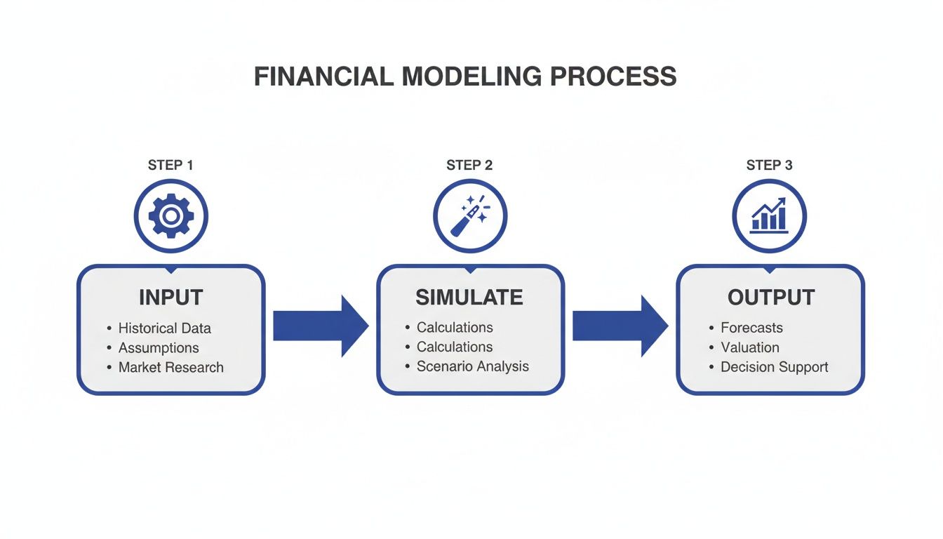
alt text: Diagram illustrating the three-step financial modeling process: Input, Simulate, and Output stages.

Here is a practical 5-step framework your team can use today.

Step 1: Model Specification

Before you write a line of code, you must define the mathematical relationship you're modeling. For simulating stock prices, the go-to starting point is Geometric Brownian Motion (GBM). This model captures two core market ideas: that stock prices follow a random walk, and that their returns—not prices—are normally distributed.

The GBM formula describes the change in a stock's price. It has two parts: a "drift" for the expected return and a "diffusion" component that introduces randomness (volatility).

Step 2: Parameter Estimation

A model is only as reliable as its data. This step, which quants call calibration, is about finding realistic values for your model’s parameters. For our GBM model, you’ll need to estimate:

• Drift (μ): The average expected return, calculated from historical daily returns.
• Volatility (σ): The standard deviation of those returns, measuring "choppiness."
• Initial Price (S₀): The asset's starting price.
• Time Horizon (T): How far you want to project (e.g., 1 year).
• Time Steps (N): The number of steps within that horizon (e.g., 252 trading days).

A common pitfall is using long-term historical averages. A better practice is to use a recent time window (1–3 years) to capture relevant market dynamics.

Step 3: Path Generation

Now you generate thousands of possible future price paths. For each time step, you inject randomness by pulling a number from a normal distribution. This random "shock" is scaled by your volatility and added to the drift to get the next price point.

This is the computationally heavy part. Using vectorized libraries like NumPy in Python is essential for getting results quickly. Modern fintech software development often parallelizes these calculations across multiple CPU cores or GPUs.

Step 4: Result Aggregation

After running, say, 10,000 simulations, you have a mountain of data. Each of the 10,000 paths represents one possible future. The job now is to consolidate that information. This typically means you'll have 10,000 different final prices, which together form a probability distribution.

Step 5: Analysis and Interpretation

With the distribution of final prices, you can answer critical business questions. What’s the probability the stock will finish above a certain price? What’s the 5th percentile outcome (a solid proxy for Value at Risk)? What’s the average expected price?

This is where the simulation proves its value. It transforms a fog of possibilities into concrete, probabilistic insights that guide investment strategy and risk management.

Practical Examples of Monte Carlo Simulation

Theory is one thing; solving real-world business problems is another. Here are two practical examples of Monte Carlo simulation in finance.

Example 1: Python Code for a Basic Stock Price Simulation

This runnable Python snippet uses NumPy to show how the 5 steps come together in code. It simulates 10,000 possible one-year price paths for a stock and calculates the expected final price and a Value at Risk (VaR) estimate.

import numpy as np# Step 2: Parameter EstimationS0 = 100      # Initial stock pricemu = 0.05     # Expected annual return (drift)sigma = 0.20  # Annual volatilityT = 1.0       # Time horizon in yearsN = 252       # Number of trading dayssimulations = 10000 # Number of simulations# Calculate time stepdt = T / N# Step 3: Path Generation (Vectorized for efficiency)# Generate random shocks for all paths and all time steps at oncerandom_shocks = np.random.normal(0, np.sqrt(dt), size=(N, simulations))# Calculate daily returnsdaily_returns = np.exp((mu - 0.5 * sigma**2) * dt + sigma * random_shocks)# Create a price path matrixprice_paths = np.zeros_like(daily_returns)price_paths[0] = S0# Generate price pathsfor t in range(1, N):price_paths[t] = price_paths[t-1] * daily_returns[t]# Step 4 & 5: Result Aggregation and Analysisfinal_prices = price_paths[-1]# Calculate key metricsexpected_price = final_prices.mean()median_price = np.median(final_prices)var_5th_percentile = np.percentile(final_prices, 5)print(f"Expected Price: ${expected_price:.2f}")print(f"5th Percentile (VaR proxy): ${var_5th_percentile:.2f}")

This code simulates 10,000 possible one-year price paths for a stock and calculates the expected final price and a 5% Value at Risk estimate.

Example 2: Mini-Case Study of a Fintech Robo-Advisor

A fintech startup launched a robo-advisor promising personalized portfolios matched to risk tolerance. The product team needs to prove their "conservative" portfolio will actually behave conservatively during a market meltdown.

The Challenge:
How does the startup prove its "conservative" portfolio can withstand a 'black swan' event? Backtesting against historical data isn't enough, as rare catastrophic events might not be in the dataset.

The Monte Carlo Solution:
The firm's quant and MLOps teams build a Monte Carlo engine to stress-test their portfolios.

1. Model the Portfolios: They define each portfolio's asset composition (e.g., US stocks, international bonds).
2. Simulate a Stress Scenario: They rig the simulation to model an extreme event. They increase volatility inputs to 40–50% (from a typical 20%), introduce a sharp negative drift to mimic a crash, and simulate a "correlation shock" where all assets fall together.
3. Run the Simulation: They run 50,000 simulations of this "black swan" scenario for each portfolio. This provides a rich distribution of potential losses.
4. Analyze and Act: The team analyzes the Conditional Value at Risk (CVaR) for each portfolio. They find their "conservative" portfolio has a 99% CVaR of -25% over one month in this nightmare scenario. This is a heavy loss but within the defined risk tolerance. By contrast, their "aggressive growth" portfolio shows a CVaR of -60%.

Business Impact:
The results are used to set honest customer expectations in the UI (e.g., "In a severe downturn, this portfolio could lose up to 25%"). It also serves as evidence for regulators, demonstrating a robust risk management framework. The time-to-value was about 3 weeks from project start to actionable risk metrics.

Deep Dive: Trade-offs, Pitfalls, and Alternatives

Monte Carlo simulation is powerful, but it's not a crystal ball. It produces probabilities, not certainties. Flawed assumptions lead to dangerously misleading conclusions and a false sense of security.

The single biggest trap is "Garbage In, Garbage Out" (GIGO). If you plug in overly optimistic return estimates or ignore recent market turmoil, the model will spit out rosy projections. This is a huge business risk.

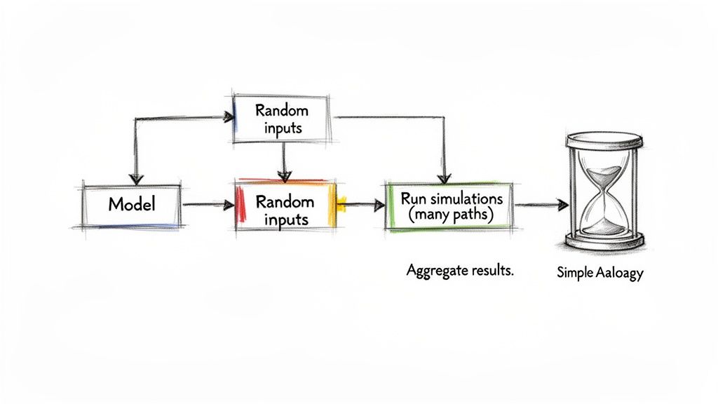
alt text: Flowchart illustrating the Monte Carlo simulation process with model, random inputs, and results aggregation.

Pitfall 1: Underestimating Tail Risk

The most common technical stumble is defaulting to the wrong statistical distribution. The normal (or Gaussian) distribution is simple but notoriously bad at capturing extreme events. Real-world financial returns have "fat tails"—catastrophic losses happen far more often than a neat bell curve predicts.

• The Problem: Using a normal distribution blinds your model to the possibility of a severe market crash.
• The Solution: Use distributions that reflect this messy reality, like the Student's t-distribution or one built from empirical data. This gives you a more honest assessment of downside risk, crucial for tasks like time-series anomaly detection.

Pitfall 2: Overlooking Computational Cost

Running millions of simulations is computationally expensive. Getting results can take too long to be useful for real-time decisions, like pricing a complex options book.

• The Problem: Standard simulations may be too slow for time-sensitive applications.
• The Solution: Use variance reduction techniques. Antithetic Variates is a simple but powerful method. For every random path your simulation generates, you create its perfect opposite. This cancels out random noise and helps the model converge faster, often achieving the same accuracy with half the simulations.

When to Use an Alternative

Monte Carlo is not always the best tool. For simple "vanilla" European options, the Black-Scholes formula is a closed-form solution that is much faster and provides an exact answer, assuming its rigid assumptions (like constant volatility) hold.

Use Monte Carlo when:

• Pricing complex, path-dependent derivatives (e.g., Asian or American options).
• Modeling portfolio-level risk with multiple, correlated assets.
• You need to account for real-world complexities like "fat tails" or shifting volatility.

Use simpler models like Black-Scholes for standard instruments where speed is critical and the model's assumptions are a reasonable fit. The key is to connect your choice of model to business impact—balancing accuracy with cost and time-to-value. This is a critical component of top financial risk management strategies.

Checklist: Is Your Monte Carlo Simulation Ready?

Use this checklist to ensure your financial models are robust, accurate, and ready for production.

Model Specification & Inputs

• Have you clearly defined the mathematical model (e.g., GBM, Heston)?
• Are your parameters (drift, volatility) calibrated with recent, relevant data?
• Have you chosen a probability distribution that accounts for fat tails (e.g., Student's t-distribution)?

Simulation & Analysis

• Have you determined the required number of simulations for convergence?
• Are you using variance reduction techniques (e.g., Antithetic Variates) to improve efficiency?
• Have you backtested the model against historical data to validate its predictive power?

Business Integration & Risk

• Are the results (e.g., VaR, CVaR) clearly translated into business impact (risk, cost)?
• Have you communicated the probabilistic nature of the forecast (e.g., "80% probability," not "guarantee") to stakeholders?
• Is there a process for regularly reviewing and recalibrating the model?

This checklist helps ensure your simulation moves from an academic exercise to a reliable tool for business decisions.

What to Do Next

1. Scope a Pilot: Use the 5-step framework to define a small-scale project. A good start is calculating the 1-day 95% VaR for a single stock portfolio.
2. Build a Proof-of-Concept: Ask an engineer to implement the Python snippet provided in this guide. This will give your team hands-on experience with the core mechanics in less than a day.
3. Book a Scoping Call: If you need to build a production-grade simulation engine, you'll need specialized talent. We can connect you with vetted senior AI and MLOps engineers who have built these systems before.

References and Further Reading

The core concepts behind Monte Carlo methods are foundational in quantitative finance. For teams looking to go deeper, we recommend starting with primary sources and official documentation for the tools you plan to use.

• Options, Futures, and Other Derivatives by John C. Hull – The definitive academic text on the models discussed.
• NumPy Documentation for numpy.random – The primary tool for generating random variables in Python.
• A deeper look at various data analysis techniques to interpret simulation outputs.

Ready to build a world-class financial product? The experts at ThirstySprout can help you hire the senior AI and MLOps engineers needed to implement robust Monte Carlo simulations and other advanced quantitative models. Start a Pilot and get matched with vetted talent in days.